I recently had the chance to use remotely sensed data to help document features of a Boulder County historic landmark, Chapman Drive. Chapman Drive is an 2.6 miles long graded unpaved road that connects Colorado State Highway 119/Boulder Canyon Road to Flagstaff Road. Chapman Drive follows the topography of the north face of Flagstaff Mountain. Chapman Drive was constructed between the fall of 1933 through spring of 1935 by the two Civilian Conservation Corps companies stationed in Boulder, Colorado (off of 6th St. and Baseline). Chapman Drive completed a scenic loop through Boulder's Mountain Parks, a corridor that contributed to the development of mountain recreation in Boulder. Thirty constructed features are associated with Chapman Drive including dry and wet laid retaining walls, cattle guards, culverts, and masonry bridges. All of these features were constructed by the Civilian Conservation Corps. You can see their skills develop throughout the roadway. By the time you reach the end of the road, it's clear that the folks that built the road, bridges, and walls are skilled craftsmen.
Disaster struck Chapman Drive in the form of historic flooding that killed 8 people and caused over $1
billion worth of damage in 14 counties in Colorado. Boulder County was one of the most severely
affected counties. During the flood, clogged drainage structures caused water to backup and carve new
drainage patterns. Massive amounts of sheetwash and gullying, segments of the road collapsing, and
a few failures of support structures resulted. The flood occurred in September 2013. The City of
Boulder is working on flood repairs for this project, which are anticipated to span end of May 2016
through first snow of autumn 2016.
As part of planning flood repairs on Chapman Drive, I completed an inventory of the affected areas.
The features of Chapman Drive had been inventoried in segments: upper Chapman Drive was
inventoried in 2009 (Feinberg and Woodham 2009) and lower Chapman Drive was inventoried in 2012
(Feinberg and Woodham 2013). Using these base data, I set to find and record Chapman Drive and its
associated features. I quickly discovered that it wasn't so easy. Nearly all of these features are
underneath the roadway on a very steep side slope. You simply can't see many of these walls from the
road or even from below the roadway. Many of the walls are broken, covered in vegetation or debris,
or simply hard to pick out from the surrounding rock outcrops. Our engineers and surveyors have
remarked at how hard it is to see the walls unless someone points them out.
My solution? Use information I already had to find these features efficiently. I am quite lucky to have
the support of a skilled GIS and information management team at Open Space and Mountain Parks
who had an existing post-flood LiDAR-derived bare earth surface model. There are five discrete
retaining wall segments in the screenshot below.
I admit that it's tough for me to clearly pick out all of the walls. In this case, I couldn't come up with
a way to consistently automatically detect wall or other relief features. There are too many similar
natural features that cause similar abrupt rises in elevation. If you used the LiDAR point cloud to
look at different returns, you could possibly automate a detection algorithm. Knowing the form and
orientation of many of these features, you would have to fit the algorithm to at least three distinct
constructions based on distance to cut, batter/slope, edge ratios, or other attributes.
Often in archaeology/cultural resource management, time and access to data are not on your side.
Instead of trying to automate something, I used the bare surface model to digitize potential historic
features before I started fieldwork. That way, I could reduce the redundancy in survey coverage and
have a feature focused tracking system. I uploaded the digitized features to a sub-meter accuracy
GPS (Trimble GeoXT 6000) and was able to compare what I saw in the LiDAR model to what I
saw on the ground in real time. This also made my evaluations of proposed treatments on historic
features easier to visualize and to communicate.
Maps made from these data showing historic feature locations, feature condition or integrity
assessments, and proposed treatment locations by treatment type were essential in showing
regulators that the project treatments were selected in interest of preservation of the overall resource.
The best use of this data was to incorporate it as well as a ground-penetrating radar survey into the
project engineering plans and specs. Our contractor, construction managers, and city staff all have
the information available as part of legally binding project documents.
Read more about Chapman Drive from Silvia Pettem, a fantastic Boulder historian.
-----------------------------------------------------------------------------------------------------------------------------
-----------------------------------------------------------------------------------------------------------------------------
Disaster struck Chapman Drive in the form of historic flooding that killed 8 people and caused over $1
billion worth of damage in 14 counties in Colorado. Boulder County was one of the most severely
affected counties. During the flood, clogged drainage structures caused water to backup and carve new
drainage patterns. Massive amounts of sheetwash and gullying, segments of the road collapsing, and
a few failures of support structures resulted. The flood occurred in September 2013. The City of
Boulder is working on flood repairs for this project, which are anticipated to span end of May 2016
through first snow of autumn 2016.
As part of planning flood repairs on Chapman Drive, I completed an inventory of the affected areas.
The features of Chapman Drive had been inventoried in segments: upper Chapman Drive was
inventoried in 2009 (Feinberg and Woodham 2009) and lower Chapman Drive was inventoried in 2012
(Feinberg and Woodham 2013). Using these base data, I set to find and record Chapman Drive and its
associated features. I quickly discovered that it wasn't so easy. Nearly all of these features are
underneath the roadway on a very steep side slope. You simply can't see many of these walls from the
road or even from below the roadway. Many of the walls are broken, covered in vegetation or debris,
or simply hard to pick out from the surrounding rock outcrops. Our engineers and surveyors have
remarked at how hard it is to see the walls unless someone points them out.
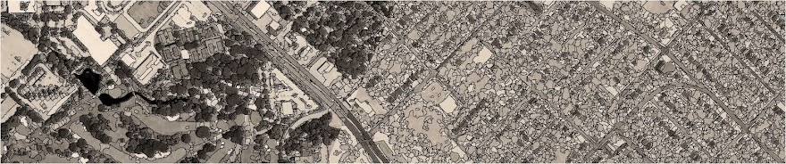
My solution? Use information I already had to find these features efficiently. I am quite lucky to have
the support of a skilled GIS and information management team at Open Space and Mountain Parks
who had an existing post-flood LiDAR-derived bare earth surface model. There are five discrete
retaining wall segments in the screenshot below.
 |
| Screenshot of post-flood LiDAR bare surface model at locations for Retaining Walls 13, 14, and 18 |
I admit that it's tough for me to clearly pick out all of the walls. In this case, I couldn't come up with
a way to consistently automatically detect wall or other relief features. There are too many similar
natural features that cause similar abrupt rises in elevation. If you used the LiDAR point cloud to
look at different returns, you could possibly automate a detection algorithm. Knowing the form and
orientation of many of these features, you would have to fit the algorithm to at least three distinct
constructions based on distance to cut, batter/slope, edge ratios, or other attributes.
Often in archaeology/cultural resource management, time and access to data are not on your side.
Instead of trying to automate something, I used the bare surface model to digitize potential historic
features before I started fieldwork. That way, I could reduce the redundancy in survey coverage and
have a feature focused tracking system. I uploaded the digitized features to a sub-meter accuracy
GPS (Trimble GeoXT 6000) and was able to compare what I saw in the LiDAR model to what I
saw on the ground in real time. This also made my evaluations of proposed treatments on historic
features easier to visualize and to communicate.
Maps made from these data showing historic feature locations, feature condition or integrity
assessments, and proposed treatment locations by treatment type were essential in showing
regulators that the project treatments were selected in interest of preservation of the overall resource.
The best use of this data was to incorporate it as well as a ground-penetrating radar survey into the
project engineering plans and specs. Our contractor, construction managers, and city staff all have
the information available as part of legally binding project documents.