Check it out! (link to full page)
.
Monday, December 11, 2017
City of Boulder Open Space & Mountain Parks Department's first Story Map!
Here it is! I have 3 more history hike narratives (written by Julie Johnson) to add to the map.
Tuesday, November 14, 2017
Close-range photogrammetry models of rock art (2/3)
Image processing and model stitching is progressing. I've been experimenting with subsetting models to maximize mesh face count and not exceeding available memory. Agisoft insists on calling subsets "chunks", which always makes me laugh as a millennial.
Here are some more recent uploads:
Head to my Sketchfab profile to see the rest and provide feedback! Stay tuned for outreach materials in the coming year.
Here are some more recent uploads:
Head to my Sketchfab profile to see the rest and provide feedback! Stay tuned for outreach materials in the coming year.
Sunday, September 3, 2017
Close-range photogrammetry models of rock art (1/3)
In fall 2016, Christian Driver and I began experimenting with close-range photogrammetry to document rock art. We help Boulder to manage rock art, specifically a series of 80+ rock art panel panels in eastern Boulder County. Many of the rock art panels in the area are too weathered to document or share satisfactorily with people. Since all of the currently detectable rock art is in relief, popular image transformations such as a principal components analysis or decorrelation are ineffective. Both of these processes are used to reduce autocorrelation (correlation of a signal with a lagged copy of itself) within a set of signals while preserving other (read: important) aspects of the signal.
- For explanation on how Dstretch works, read Dr. Ronald E. Alley's white paper. Before reading Dr. Alley's paper, I didn't realize that the Jet Propulsion Lab developed the algorithm used by Dstretch originally for ASTER, a 14-band multispectral sensor. I'm interested in learning more about how dramatically fewer data points in typical RGB camera sensors used for rock art change the dimensionality of the algorithm.
While the spectral information of the rock art itself is not sufficiently different than that of the surrounding rock to distinguish the rock art, the spatial information of the rock art is sufficiently different than that of the surrounding rock to distinguish it if you can capture it. Traditional rock art documentation was completed between 1984 and 1997 by the Indian Peaks chapter of the Colorado Archaeological Society (Kindig 1997). These recordings, while infinitely valuable for identification and relocation of panels, have a few limitations. They are not to scale, do not capture the type or method of rock art creation, do not capture condition or imminent threats (cracks, sloughing, vandalism, infiltration), and do not document the surrounding rock surface (texture, bedding, color, shape/volume). What data model maximizes production of these data for the least amount of time and cost? 3-dimensional or 3D models is a great start.
There are several ways to capture these 3D data, many of them are demonstrably "whiz-bang" as many of my bosses say. Terrestrial laser scanners are the fastest and most expensive method we found, which maximizes spatial extent and spatial differences but is less effective in capturing spectral information. We focused on close-range photogrammetry for several reasons: it's fast, it's cheap (price of sufficient quality DSLR camera (thanks Christian!), lenses (usually 50mm), and software unless open source), spectral, spatial, textural data captures are sufficient resolution, and it's reproducible.
Check out some examples of our 3D models so far. The models are color balanced and to scale. Sometimes the spatial extent of data capture is limited by our computer processing capacity. I'm hoping to experiment with parallel processing/RAM and processor upgrades in the next few months.
Please leave me comments on either this page or Sketchfab if you enjoy seeing the models, what you did and did not like about the models, and any changes you suggest.
-------------------------------------------------------------------------------------------------------------
Oil derrick
"Kirkendoll"
"WFM/ 1904"
Friday, March 31, 2017
DATA SHARE: Boulder local landmarks, historic districts, State and National Register listed resources
As part of a new planning effort at work, I assembled geospatial data for designated historic properties in City of Boulder and its public lands (45,000 acres surrounding Boulder, Colorado). These data were aggregated from:
- City of Boulder historic landmarks and districts (excluding contributing elements and potential districts),
- Boulder County historic landmarks,
- Boulder County historic districts and cultural landscapes,
- Colorado State Register of Historic Places-listed properties,
- National Register of Historic Places-listed properties, and
- National Historic Landmarks.
You can download this zip file, which contains an ESRI Layer Package file and accompanying shapefile of assembled info. The EPSG is 2876. Metadata is FGDC compliant and documents data sources, limits, and processing. Tabular data include designation type, parcel number, resource name.
NOTE: These data do not include protected information and are publicly available from their respective sources (City of Boulder, Boulder County, Colorado Office of Archaeology and Historic Preservation, and National Park Service).
Thursday, February 2, 2017
Saving Places 2017 Presentation
In February 2017, I presented at Colorado Preservation Inc.'s Saving Places Conference about using geospatial data to study linear cultural resources. The slideshow is accessible here for those looking for geospatial data (remotely sensed particularly) sources as promised.
This presentation was prompted by a paucity of evidence from existing and free geospatial data in cultural resource management reports and resource forms. Given the deposition context of the Front Range of Colorado where you can find both prehistoric and historic components on the ground surface, CRM archaeologists are missing out on time efficient and defensible data sources for resource documentation. Linear resources especially benefit from a geospatial approach because they're usually often difficult to record in entirety and assess segment contribution to overall resource eligibility to the National Register of Historic Places and a geospatial approach gives the CRM archaeologist basic lines of evidence to generate recommendations based on integrity (NPS Guidelines on Evaluating Integrity).
My goal for this presentation was to give the audience questions to ask of existing geospatial data to inform evaluations of cultural resource integrity and historic significance. The questions increase in specificity from broad (What is my geographic area of interest?) to pointed (Have design, setting, associations changed?) to concurring data (Do multiple sources agree?). I show examples from my own work in Boulder featuring:
Feel free to contact me with questions about the materials. I'm always happy to help people get the most out of their time and money/free data.
-Katy
This presentation was prompted by a paucity of evidence from existing and free geospatial data in cultural resource management reports and resource forms. Given the deposition context of the Front Range of Colorado where you can find both prehistoric and historic components on the ground surface, CRM archaeologists are missing out on time efficient and defensible data sources for resource documentation. Linear resources especially benefit from a geospatial approach because they're usually often difficult to record in entirety and assess segment contribution to overall resource eligibility to the National Register of Historic Places and a geospatial approach gives the CRM archaeologist basic lines of evidence to generate recommendations based on integrity (NPS Guidelines on Evaluating Integrity).
My goal for this presentation was to give the audience questions to ask of existing geospatial data to inform evaluations of cultural resource integrity and historic significance. The questions increase in specificity from broad (What is my geographic area of interest?) to pointed (Have design, setting, associations changed?) to concurring data (Do multiple sources agree?). I show examples from my own work in Boulder featuring:
- spectral information using multispectral aerial imagery with band indices,
- texture using high spatial resolution panchromatic satellite imagery,
- historic-age maps (from Civilian Conservation Corps in Boulder, 1935),
- LiDAR point clouds,
- LiDAR digital elevation models (DEM),
- LiDAR digital surface models (DSM), and
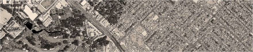
- change detection using panchromatic historical orthorectified and oblique aerial imagery (partial example below).
Feel free to contact me with questions about the materials. I'm always happy to help people get the most out of their time and money/free data.
-Katy
Friday, September 2, 2016
Interview with new Colorado Assistant State Archaeologist, Chris Johnston
Stay up to date with History Colorado's Blogs for interesting pieces on national, state, and local archaeological and preservation topics.
Monday, June 27, 2016
Viewshed and visual impacts assessment near Colorado Chautuaqua, Boulder, Colorado
One of the most distinctive areas of Boulder is the Colorado Chautauqua, located on the edge of Enchanted Mesa overlooking the Boulder Valley. It has served as a rural enclave to urban Boulder since 1898. The Colorado Chautauqua has provided a variety of programs for over a century, including concerts, debates, lectures, and other recreational activities. Read more about the offerings of the Colorado Chautauqua in Mary Galey's The Grand Assembly, considered the authoritative text on the Colorado Chautauqua.
Recently, Open Space and Mountain Parks Department (land managers for Chautauqua Meadow and lands surrounding Colorado Chautauqua) proposed repairs to the Chautauqua Trail. Chautauqua Trail is the flagship trail that most visitors (over 3 million annually) hike during their visit to Chautauqua Meadow or Colorado Chautauqua. The current trail design is problematic and leads visitors to hike off trail, causing braiding, erosion, and expansion of the trail corridor. The trail was maintained to be 8 feet wide; it is currently 24 feet wide in spots (Figure 1). Additionally, there are several informal gathering areas where folks like to take photos with the Flatirons in the background. Open Space and Mountain Parks would like to improve the trail by stabilizing the trail tread and to designate low development level gathering areas to minimize existing resource damage.
During the planning phase of this and similar projects, we consult with neighbors and stakeholders on the proposed work. One stakeholder was particularly concerned that our trail work would negatively impact the viewshed of Colorado Chautauqua. In response to the concern, my crew devised a two part plan to assess the viewshed impacts to Colorado Chautauqua.
1. 3D Viewshed Model
I constructed 3D viewshed models with ArcGIS 10.4 of the lines of sight from our treatment locations (Figure 2), key observation points identified by the stakeholder (Figure 3), and key observation points identified by Open Space and Mountain Parks (Figure 4). These locations are listed below. The viewshed models were generated using a 1 foot spatial resolution digital surface model (DSM) that included obstacles (buildings, vegetation). The DSM was derived from post-flood aerial LiDAR point cloud for the City of Boulder. The height of the observer was chosen at 6 feet above ground surface, simulating the viewshed for taller individuals to maximize the visibility of surrounding features.
Creating 3D viewsheds in a geographic information system (GIS) have benefits and drawbacks compared to other methods of viewshed assessment. A GIS is better able to consider the effects of terrain relief and curvature of the earth, creating a quantifiable output of what areas are visible or not from a given location. Because of Earth's curvature, lines of sight can only extend up to 3 miles or 5 kilometers unless drastic changes in elevation are involved. A GIS makes it easier to assess object and observer heights. Our models did not consider atmospheric refraction and how visibility of an object is affected. The GIS models also do not address observer's visual acuity. An object may have a clear line of sight to an observer, but an observer may not have the ability to see that object.
Visualizations from the model illustrate the results. The viewshed model for our proposed treatment locations shows that little of the landmark shares clear lines of sight with the treatment locations (Figure 2). The viewshed from Colorado Chautauqua is not substantially impacted (Figure 3). In assessing the potential for adverse indirect effects of our proposed treatments, we expect that no areas of concern at Colorado Chautauqua showed potential for adverse effects. The viewshed towards Colorado Chautauqua from the Chautauqua Meadow is likely to be impacted by the proposed treatments (Figure 4). There are clear lines of sight from one key observation point at each gathering area.
_________________________________________________________________________________
2. Visual Contrast Rating Survey
The second part of our approach to demonstrate the potential impacts on the viewshed of Colorado Chautauqua was to conduct a Visual Contrast Rating (VCR) Survey. This survey was organized by my co-worker (fellow OSMP archaeologist), Christian Driver. We used a modified format of the Bureau of Land Management's inventory form. The purpose of a VCR survey is to analyze potential visual impact of proposed projects and activities. It requires participants to apply the basic principles of design in the resolution of visual impacts. The VCR survey process provides a means for determining visual impacts and for identifying measures to mitigate these impacts.
History of the Colorado Chautauqua
In the late 1890s, a group of Texans (including University of Texas president G. F. Winston) wanted to open up their own Chautauqua and looked to the Rocky Mountains for a location. Boulder was chosen for the site of Chautauqua and Boulder citizens, thrilled to have a Chautauqua nearby, raised $20,000 towards construction costs. The city of Boulder purchased 171 acres from the Bachelder Ranch and the Austin-Russel tract for the new Chautauqua, the first purchase of private property by the city of Boulder. The Texans covered expenses of running the Chautauqua programs.
 |
| "The First Chautauqua at Boulder, Colo. 1898. Texas-Colorado Chautauqua, looking west. H. F. Pierson photo, Denver, Colo." Boulder Carnegie Library for Local History, 511-3-9 PHOTO 1. |
The Colorado Chautauqua was part of the national Chautauqua movement, which was nationally known for its emphasis on intellectual pursuits, moral self-improvement, and civic involvement. The movement began in upstate New York in 1876 as a center for political, educational, and recreational programs. By 1924, nearly 40 million people were annually attending events at over 300 Chautauquas across the country. The Chautauqua movement died out by the mid-1930s. Most historians cite the rise of car culture, radio, and movies among the primary causes as well as social changes, including a sharp increase in fundamentalism and evangelical Christianity in the 1920s, alternative educational opportunities for women, and the economic impossibility of organizing programs. Many Chautauqua communities became camp meetings or church camps.
By 1955, Boulder's Chautauqua was one of only six remaining in the country. The programs and activities continued at the Colorado Chautauqua as they had since the beginning, but many of the building began to deteriorate. By 1975, the city of Boulder considered tearing the buildings down, but concern about the future of the park inspired the citizens of Boulder and the Colorado Chautauqua Association to implement a program to preserve the park and its historic buildings, structures, and landscape. In 1978, Colorado Chautauqua was designated as a local historic district and was listed on the National Register of Historic Places. In 2006, Colorado Chautauqua was designated as a National Historic Landmark.
Managing the Viewshed of the Colorado Chautauqua
Recently, Open Space and Mountain Parks Department (land managers for Chautauqua Meadow and lands surrounding Colorado Chautauqua) proposed repairs to the Chautauqua Trail. Chautauqua Trail is the flagship trail that most visitors (over 3 million annually) hike during their visit to Chautauqua Meadow or Colorado Chautauqua. The current trail design is problematic and leads visitors to hike off trail, causing braiding, erosion, and expansion of the trail corridor. The trail was maintained to be 8 feet wide; it is currently 24 feet wide in spots (Figure 1). Additionally, there are several informal gathering areas where folks like to take photos with the Flatirons in the background. Open Space and Mountain Parks would like to improve the trail by stabilizing the trail tread and to designate low development level gathering areas to minimize existing resource damage.
 |
| Figure 1. Photo CT.7785: Overview of Chautauqua Trail below/northeast of Gathering Area 2 (GA2) looking northeast towards Colorado Chautauqua. Braiding, gullying, weed encroachment visible on trail. |
1. 3D Viewshed Model
I constructed 3D viewshed models with ArcGIS 10.4 of the lines of sight from our treatment locations (Figure 2), key observation points identified by the stakeholder (Figure 3), and key observation points identified by Open Space and Mountain Parks (Figure 4). These locations are listed below. The viewshed models were generated using a 1 foot spatial resolution digital surface model (DSM) that included obstacles (buildings, vegetation). The DSM was derived from post-flood aerial LiDAR point cloud for the City of Boulder. The height of the observer was chosen at 6 feet above ground surface, simulating the viewshed for taller individuals to maximize the visibility of surrounding features.
Creating 3D viewsheds in a geographic information system (GIS) have benefits and drawbacks compared to other methods of viewshed assessment. A GIS is better able to consider the effects of terrain relief and curvature of the earth, creating a quantifiable output of what areas are visible or not from a given location. Because of Earth's curvature, lines of sight can only extend up to 3 miles or 5 kilometers unless drastic changes in elevation are involved. A GIS makes it easier to assess object and observer heights. Our models did not consider atmospheric refraction and how visibility of an object is affected. The GIS models also do not address observer's visual acuity. An object may have a clear line of sight to an observer, but an observer may not have the ability to see that object.
Visualizations from the model illustrate the results. The viewshed model for our proposed treatment locations shows that little of the landmark shares clear lines of sight with the treatment locations (Figure 2). The viewshed from Colorado Chautauqua is not substantially impacted (Figure 3). In assessing the potential for adverse indirect effects of our proposed treatments, we expect that no areas of concern at Colorado Chautauqua showed potential for adverse effects. The viewshed towards Colorado Chautauqua from the Chautauqua Meadow is likely to be impacted by the proposed treatments (Figure 4). There are clear lines of sight from one key observation point at each gathering area.
 |
| Figure 2: Lines of sight from proposed gathering areas. Gathering areas construction will require application of StaLok surfacing and irregular placement of boulders to delineate from off-trail terrain. Cells in green are visible from both gathering areas, blue cells are visible from one gathering area, uncolored cells are not visible from any proposed gathering area. |
 |
| Figure 3: Lines of sight from stakeholder-identified key observation points. Cells are color coded for how many key observation points have clear lines of sight to them. |
 |
| Figure 4: Lines of sight from Open Space and Mountain Parks-identified key observation points. Cells are color coded for how many key observation points have clear lines of sight to them. |
_________________________________________________________________________________
DESCRIPTIONS OF KEY OBSERVATION POINTS:
| CCA1: | Vehicle entry at Kinikinik Road | OSMP1: | 7th Street and Baseline | GA1: | Gathering Area 1 | ||
| CCA2: | Chautauqua Green | OSMP2: | Divergence of Baseline and Flagstaff Road | GA2: | Gathering Area 2 | ||
| CCA3: | Gwenthean Cottage | OSMP3: | Armstrong Bridge | ||||
| CCA4: | Chautauqua Arbor | OSMP4: | Ski Jump Trail at woodland edge | ||||
| CCA5: | Bluebell Road (Cottage 26) | OSMP5: | Chautauqua Trail and Bluebell Mesa Trail | ||||
| CCA6: | Columbine Lodge (west hallway on 2nd floor) | OSMP6: | Bluebell Mesa Trail at woodland edge | ||||
| CCA7: | Columbine Lodge (northern elevation porch on 2nd floor) | OSMP7: | Bluebell Road (near Cottage 811) | ||||
| CCA8: | Cottage 16 | OSMP8: | Meadow Trail near Civilian Conservation Corps site |
2. Visual Contrast Rating Survey
 |
| Figure 6: Triangular 12 inches by 6 inches target. Targets were placed in proposed gathering areas. |
 |
| Figure 7: Subset of VCR survey group, including OSMP trail project manager, archaeologist, and Colorado Chautauqua Association Facilities Manager |
The VCR methods holds that degree to which a management activity/treatment affects the visual quality of a landscape depends on the visual contrast created between a project and the existing landscape. The contrast can be measured by comparing the project features with the major features in the existing landscape. The basic design elements of form, line, color, and texture are used to make this comparison and to describe the visual contrast created by the project.
A VCR survey was completed in two days by four people, including a representative from the concerned stakeholder. Data and findings are still being compiled from the inventory forms. Discussions during the survey found consensus in how few of the treatment areas were actually visible by our own sight from key observation points.
Consultation for this project is still ongoing with 30% Plan Sheets anticipated to be released in the next few weeks. I will update this post periodically as we advance in the planning process, particularly as we may need to seek additional clearances with a local landmark board to proceed. This viewshed analysis and visual resource assessment provided robust framework for conversations about indirect effects to significant historic properties. I consider this process successful in achieving our goals.
Monday, April 11, 2016
ArchaeoTech Podcast: Photogrammetry and Field Photography
The ArchaeoTech podcast (Archaeology Podcast Network) has put out another great episode on one of my favorite digital tools, photogrammetry. Dr. Michael Ashley of Codifi and the Center for Digital Archaeology is the featured guest.
Check it out: Photogrammetry and Great Field Photography
Wednesday, February 10, 2016
Entitlement in cultural resource management job hunting
Check out this great post from Bill White of Succinct Research on job hunting and recent graduate entitlement:
I have seen what Bill discusses in both undergraduate and graduate folks. I agree that the entitled attitude is not usually successful in helping folks land jobs. On the other hand, I've seen and continue to see overqualified folks take jobs well under their pay grade and skill set. There's nothing wrong with working as a technician when you have advanced skills and experience as long as that's the job you agreed to perform. There are many things wrong with classifying and paying your project manager or principal investigator as a technician. Don't get me started on agencies/firms that advertise a position at a lower grade than the work they want done.
Monday, December 28, 2015
ArchaeoTech Podcast: 3D Scanning
The ArchaeoTech podcast (Archaeology Podcast Network) has put out a great episode on 3D scanning and printing. Bernard Means, Director of the Virtual Curation Laboratory at Virginia Commonwealth University, is the featured guest.
Check it out: 3D Printing and Scanning
Saturday, August 29, 2015
Remote sensing to document historic features at Chapman Drive, Boulder County, Colorado
I recently had the chance to use remotely sensed data to help document features of a Boulder County historic landmark, Chapman Drive. Chapman Drive is an 2.6 miles long graded unpaved road that connects Colorado State Highway 119/Boulder Canyon Road to Flagstaff Road. Chapman Drive follows the topography of the north face of Flagstaff Mountain. Chapman Drive was constructed between the fall of 1933 through spring of 1935 by the two Civilian Conservation Corps companies stationed in Boulder, Colorado (off of 6th St. and Baseline). Chapman Drive completed a scenic loop through Boulder's Mountain Parks, a corridor that contributed to the development of mountain recreation in Boulder. Thirty constructed features are associated with Chapman Drive including dry and wet laid retaining walls, cattle guards, culverts, and masonry bridges. All of these features were constructed by the Civilian Conservation Corps. You can see their skills develop throughout the roadway. By the time you reach the end of the road, it's clear that the folks that built the road, bridges, and walls are skilled craftsmen.
Disaster struck Chapman Drive in the form of historic flooding that killed 8 people and caused over $1
billion worth of damage in 14 counties in Colorado. Boulder County was one of the most severely
affected counties. During the flood, clogged drainage structures caused water to backup and carve new
drainage patterns. Massive amounts of sheetwash and gullying, segments of the road collapsing, and
a few failures of support structures resulted. The flood occurred in September 2013. The City of
Boulder is working on flood repairs for this project, which are anticipated to span end of May 2016
through first snow of autumn 2016.
As part of planning flood repairs on Chapman Drive, I completed an inventory of the affected areas.
The features of Chapman Drive had been inventoried in segments: upper Chapman Drive was
inventoried in 2009 (Feinberg and Woodham 2009) and lower Chapman Drive was inventoried in 2012
(Feinberg and Woodham 2013). Using these base data, I set to find and record Chapman Drive and its
associated features. I quickly discovered that it wasn't so easy. Nearly all of these features are
underneath the roadway on a very steep side slope. You simply can't see many of these walls from the
road or even from below the roadway. Many of the walls are broken, covered in vegetation or debris,
or simply hard to pick out from the surrounding rock outcrops. Our engineers and surveyors have
remarked at how hard it is to see the walls unless someone points them out.
My solution? Use information I already had to find these features efficiently. I am quite lucky to have
the support of a skilled GIS and information management team at Open Space and Mountain Parks
who had an existing post-flood LiDAR-derived bare earth surface model. There are five discrete
retaining wall segments in the screenshot below.
I admit that it's tough for me to clearly pick out all of the walls. In this case, I couldn't come up with
a way to consistently automatically detect wall or other relief features. There are too many similar
natural features that cause similar abrupt rises in elevation. If you used the LiDAR point cloud to
look at different returns, you could possibly automate a detection algorithm. Knowing the form and
orientation of many of these features, you would have to fit the algorithm to at least three distinct
constructions based on distance to cut, batter/slope, edge ratios, or other attributes.
Often in archaeology/cultural resource management, time and access to data are not on your side.
Instead of trying to automate something, I used the bare surface model to digitize potential historic
features before I started fieldwork. That way, I could reduce the redundancy in survey coverage and
have a feature focused tracking system. I uploaded the digitized features to a sub-meter accuracy
GPS (Trimble GeoXT 6000) and was able to compare what I saw in the LiDAR model to what I
saw on the ground in real time. This also made my evaluations of proposed treatments on historic
features easier to visualize and to communicate.
Maps made from these data showing historic feature locations, feature condition or integrity
assessments, and proposed treatment locations by treatment type were essential in showing
regulators that the project treatments were selected in interest of preservation of the overall resource.
The best use of this data was to incorporate it as well as a ground-penetrating radar survey into the
project engineering plans and specs. Our contractor, construction managers, and city staff all have
the information available as part of legally binding project documents.
Read more about Chapman Drive from Silvia Pettem, a fantastic Boulder historian.
-----------------------------------------------------------------------------------------------------------------------------
-----------------------------------------------------------------------------------------------------------------------------
Disaster struck Chapman Drive in the form of historic flooding that killed 8 people and caused over $1
billion worth of damage in 14 counties in Colorado. Boulder County was one of the most severely
affected counties. During the flood, clogged drainage structures caused water to backup and carve new
drainage patterns. Massive amounts of sheetwash and gullying, segments of the road collapsing, and
a few failures of support structures resulted. The flood occurred in September 2013. The City of
Boulder is working on flood repairs for this project, which are anticipated to span end of May 2016
through first snow of autumn 2016.
As part of planning flood repairs on Chapman Drive, I completed an inventory of the affected areas.
The features of Chapman Drive had been inventoried in segments: upper Chapman Drive was
inventoried in 2009 (Feinberg and Woodham 2009) and lower Chapman Drive was inventoried in 2012
(Feinberg and Woodham 2013). Using these base data, I set to find and record Chapman Drive and its
associated features. I quickly discovered that it wasn't so easy. Nearly all of these features are
underneath the roadway on a very steep side slope. You simply can't see many of these walls from the
road or even from below the roadway. Many of the walls are broken, covered in vegetation or debris,
or simply hard to pick out from the surrounding rock outcrops. Our engineers and surveyors have
remarked at how hard it is to see the walls unless someone points them out.
My solution? Use information I already had to find these features efficiently. I am quite lucky to have
the support of a skilled GIS and information management team at Open Space and Mountain Parks
who had an existing post-flood LiDAR-derived bare earth surface model. There are five discrete
retaining wall segments in the screenshot below.
 |
| Screenshot of post-flood LiDAR bare surface model at locations for Retaining Walls 13, 14, and 18 |
I admit that it's tough for me to clearly pick out all of the walls. In this case, I couldn't come up with
a way to consistently automatically detect wall or other relief features. There are too many similar
natural features that cause similar abrupt rises in elevation. If you used the LiDAR point cloud to
look at different returns, you could possibly automate a detection algorithm. Knowing the form and
orientation of many of these features, you would have to fit the algorithm to at least three distinct
constructions based on distance to cut, batter/slope, edge ratios, or other attributes.
Often in archaeology/cultural resource management, time and access to data are not on your side.
Instead of trying to automate something, I used the bare surface model to digitize potential historic
features before I started fieldwork. That way, I could reduce the redundancy in survey coverage and
have a feature focused tracking system. I uploaded the digitized features to a sub-meter accuracy
GPS (Trimble GeoXT 6000) and was able to compare what I saw in the LiDAR model to what I
saw on the ground in real time. This also made my evaluations of proposed treatments on historic
features easier to visualize and to communicate.
Maps made from these data showing historic feature locations, feature condition or integrity
assessments, and proposed treatment locations by treatment type were essential in showing
regulators that the project treatments were selected in interest of preservation of the overall resource.
The best use of this data was to incorporate it as well as a ground-penetrating radar survey into the
project engineering plans and specs. Our contractor, construction managers, and city staff all have
the information available as part of legally binding project documents.
Monday, February 16, 2015
Primer on ground-penetrating radar
Ground-penetrating radar (GPR) is a geophysical method that uses radar pulses to image the subsurface. This nondestructive method uses electromagnetic radiation in the microwave band (UHF/VHF frequencies) of the electromagnetic spectrum, and detects the reflected signals from subsurface structures. GPR can have applications in a variety of media, including rock, soil, ice, fresh water, pavements and structures. In the right conditions, practitioners can use GPR to detect subsurface objects, changes in material properties, and voids and cracks. Ground-penetrating radar antennas are generally put into contact with the ground for the strongest signal strength. However, airborne GPR antennas can be used above the ground. I have no experience with airborne GPR and will not speak to them.

Think about times when you've seen GPR surveys presented in magazine articles or other publications. Most of those maps used are amplitude slice or slice maps. The maps show horizontal "slices" of the entire survey area from a specific travel time (not necessarily same depth). They typically feature bright or two tone colormaps. The colors represent the amplitude of a trace or waveform at that particular travel time. Amplitude is important as is visualizing the data on a horizontal plane, but amplitudes alone can't be interpreted as features. I will discuss more on waveform amplitude and associated issues at a later date. They are visually attractive and understandably very common in media and publications.
_________________________________________________________________________
GPR Basics:
GPR transmitter emits electromagnetic energy into the ground. When the energy encounters a buried object or a boundary between materials having different dielectric constants (also referred to as relative dielectric permittivity), it may be reflected or refracted or scattered back to the surface. A receiving antenna can then record the variations in the return signal. The principles involved are similar to seismology, except that electromagnetic energy is used instead of acoustic energy, and energy may be reflected at boundaries where subsurface electrical properties change rather than subsurface mechanical properties as is the case with seismic energy. The key to detecting features with GPR is that there must be compositional differences between the object, feature, or materials of interest relative to their surrounding media.
GPR transmits electromagnetic pulses from surface antennas into the ground, and then measures the time elapsed between when the pulses are sent and when they are received back at the surface (Conyers and Goodman 1997). Each pulse emitted from the antenna is recorded as an individual trace, which can be referenced as distance or location along a survey transect. So if there's a feature of interest that you see in a radar profile (looking at a cross section of the ground, e.g. not planar map), you can refer to Trace number ____ and use the known length of the transect to figure out the planar location of the feature. Thankfully all GPR data viewing software I know of calculate this for you. Radar travel times (think vertical now) are measured in nanoseconds. So if there's a feature of interest that you see in a radar profile (looking at a cross section of the ground, e.g. not planar map), you can refer to the travel time (___ nanoseconds) and calculate the distance between ground surface and the subsurface feature (using velocity). This is not automatically calculated unless you are able to determine what kind of media the energy is traveling through. If you know the media, you can use known rates of travel (relative dielectric permittivity) to calculate distance from the ground surface. The ability to give each reflection precise depth information is not available in other shallow geophysical methods, which is tremendously useful. GPR surveys allow for a relatively wide aerial coverage in a short period of time, with excellent spatial resolution of buried archaeological features and their related stratigraphy.
Back to radar physics:
Radar waves that move in both the air and the ground are a form of electromagnetic energy composed of cojoined oscillating electrical and magnetic fields. GPR uses high-frequency radio waves (usually polarized) in the range 10 MHz to 1 GHz. These waves are produced when an electric current oscillates back and forth in a conductive body, producing a subsidiary magnetic field. EM waves are then generated that propagate outward from the source. Radar energy used in GPR is produced at an antenna, the simplest of which is a copper wire or plate on which an oscillating electrical current is applied. Depending on the frequency of the oscillation (measured in cycles per second, hertz unit), different wavelengths of propagating radar waves are produced. Different frequency antennas give you different results. Low frequency (~100-200 MHz) and very low frequency (<100 MHz) antennas are suitable for large extent geological or geomorphological features (large scale/low detail). Medium frequency antennas (~200-800 MHz) are suitable for most archaeological applications. Depending on the soils, medium frequency antennas can yield horizontal resolution of as little as 10 cm and vertical resolution as little as 16 cm (in case of dry sand). High frequency antennas (>800 MHz) are suitable for detecting smaller and shallower features where you already know or suspect they are located. The resolution capability increases as center mean frequency of antennas increase; beware of lower depth penetration and shallower attenuation (signal deteriorates into noise) with higher frequency antennas.
The electrical conductivity of the ground, the transmitted center frequency, and the power of the transmitted energy all may limit the effective depth range of GPR investigation. Increases in electrical conductivity attenuate the introduced electromagnetic wave, and thus the penetration depth decreases. Higher frequencies do not penetrate as far as lower frequencies. However, higher frequencies provide improved resolution. Thus operating frequency is always a trade-off between resolution and penetration. Optimal depth of subsurface penetration is achieved in ice where the depth of penetration can achieve several thousand meters (to bedrock in Greenland) at low GPR frequencies. Dry sandy soils or massive dry materials such limestone, and concrete tend to be resistive rather than conductive, and the depth of penetration could be up to 15 meters. In moist and/or clay-laden soils (especially four layer clays like kaolin and smectite groups) and materials with high electrical conductivity, penetration may be as little as a few centimeters.
What is a radar profile or radargram?
As the antennas are moved along the ground surface, individual reflections are recorded about every 2 to 10 centimeters along transects. The form of the individual reflected waves (called a waveform) that are received from within the ground is then digitized into a reflection trace, which is a series of waves reflected back to one surface location. When many traces are stacked next to each other sequentially, a two-dimensional vertical profile is produced along a transect over which the antenna was moved: a GPR reflection profile. This shows how, where, and how much the energy was reflected or traveled through the ground in a cross-section of the ground along a horizontal plane. For archaeologists, think of it as an excavation unit wall: you can see vertical layering and (sometimes) horizons.
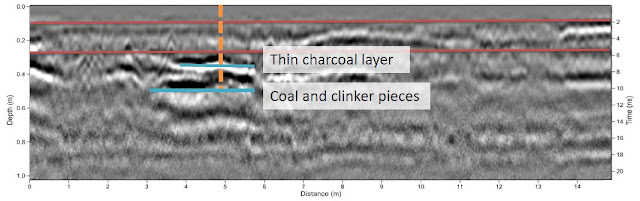
As a GPR practioner, I get nearly all of the information I use for interpretation of GPR data from radar profiles. Profiles give you much more information about the orientation, shape, continuity, and compositional differences of the subsurface materials than an amplitude slice or slice maps.
GPR transmitter emits electromagnetic energy into the ground. When the energy encounters a buried object or a boundary between materials having different dielectric constants (also referred to as relative dielectric permittivity), it may be reflected or refracted or scattered back to the surface. A receiving antenna can then record the variations in the return signal. The principles involved are similar to seismology, except that electromagnetic energy is used instead of acoustic energy, and energy may be reflected at boundaries where subsurface electrical properties change rather than subsurface mechanical properties as is the case with seismic energy. The key to detecting features with GPR is that there must be compositional differences between the object, feature, or materials of interest relative to their surrounding media.
GPR transmits electromagnetic pulses from surface antennas into the ground, and then measures the time elapsed between when the pulses are sent and when they are received back at the surface (Conyers and Goodman 1997). Each pulse emitted from the antenna is recorded as an individual trace, which can be referenced as distance or location along a survey transect. So if there's a feature of interest that you see in a radar profile (looking at a cross section of the ground, e.g. not planar map), you can refer to Trace number ____ and use the known length of the transect to figure out the planar location of the feature. Thankfully all GPR data viewing software I know of calculate this for you. Radar travel times (think vertical now) are measured in nanoseconds. So if there's a feature of interest that you see in a radar profile (looking at a cross section of the ground, e.g. not planar map), you can refer to the travel time (___ nanoseconds) and calculate the distance between ground surface and the subsurface feature (using velocity). This is not automatically calculated unless you are able to determine what kind of media the energy is traveling through. If you know the media, you can use known rates of travel (relative dielectric permittivity) to calculate distance from the ground surface. The ability to give each reflection precise depth information is not available in other shallow geophysical methods, which is tremendously useful. GPR surveys allow for a relatively wide aerial coverage in a short period of time, with excellent spatial resolution of buried archaeological features and their related stratigraphy.
Back to radar physics:
Radar waves that move in both the air and the ground are a form of electromagnetic energy composed of cojoined oscillating electrical and magnetic fields. GPR uses high-frequency radio waves (usually polarized) in the range 10 MHz to 1 GHz. These waves are produced when an electric current oscillates back and forth in a conductive body, producing a subsidiary magnetic field. EM waves are then generated that propagate outward from the source. Radar energy used in GPR is produced at an antenna, the simplest of which is a copper wire or plate on which an oscillating electrical current is applied. Depending on the frequency of the oscillation (measured in cycles per second, hertz unit), different wavelengths of propagating radar waves are produced. Different frequency antennas give you different results. Low frequency (~100-200 MHz) and very low frequency (<100 MHz) antennas are suitable for large extent geological or geomorphological features (large scale/low detail). Medium frequency antennas (~200-800 MHz) are suitable for most archaeological applications. Depending on the soils, medium frequency antennas can yield horizontal resolution of as little as 10 cm and vertical resolution as little as 16 cm (in case of dry sand). High frequency antennas (>800 MHz) are suitable for detecting smaller and shallower features where you already know or suspect they are located. The resolution capability increases as center mean frequency of antennas increase; beware of lower depth penetration and shallower attenuation (signal deteriorates into noise) with higher frequency antennas.
The electrical conductivity of the ground, the transmitted center frequency, and the power of the transmitted energy all may limit the effective depth range of GPR investigation. Increases in electrical conductivity attenuate the introduced electromagnetic wave, and thus the penetration depth decreases. Higher frequencies do not penetrate as far as lower frequencies. However, higher frequencies provide improved resolution. Thus operating frequency is always a trade-off between resolution and penetration. Optimal depth of subsurface penetration is achieved in ice where the depth of penetration can achieve several thousand meters (to bedrock in Greenland) at low GPR frequencies. Dry sandy soils or massive dry materials such limestone, and concrete tend to be resistive rather than conductive, and the depth of penetration could be up to 15 meters. In moist and/or clay-laden soils (especially four layer clays like kaolin and smectite groups) and materials with high electrical conductivity, penetration may be as little as a few centimeters.
What is a radar profile or radargram?
As the antennas are moved along the ground surface, individual reflections are recorded about every 2 to 10 centimeters along transects. The form of the individual reflected waves (called a waveform) that are received from within the ground is then digitized into a reflection trace, which is a series of waves reflected back to one surface location. When many traces are stacked next to each other sequentially, a two-dimensional vertical profile is produced along a transect over which the antenna was moved: a GPR reflection profile. This shows how, where, and how much the energy was reflected or traveled through the ground in a cross-section of the ground along a horizontal plane. For archaeologists, think of it as an excavation unit wall: you can see vertical layering and (sometimes) horizons.

Radar reflection profile from University of Denver Humanities Garden survey (2013)
As a GPR practioner, I get nearly all of the information I use for interpretation of GPR data from radar profiles. Profiles give you much more information about the orientation, shape, continuity, and compositional differences of the subsurface materials than an amplitude slice or slice maps.
What are slice maps?

Amplitude slices at 5 nanosecond increments from Humanities Garden survey (2013); 400 MHz frequency antennas
Think about times when you've seen GPR surveys presented in magazine articles or other publications. Most of those maps used are amplitude slice or slice maps. The maps show horizontal "slices" of the entire survey area from a specific travel time (not necessarily same depth). They typically feature bright or two tone colormaps. The colors represent the amplitude of a trace or waveform at that particular travel time. Amplitude is important as is visualizing the data on a horizontal plane, but amplitudes alone can't be interpreted as features. I will discuss more on waveform amplitude and associated issues at a later date. They are visually attractive and understandably very common in media and publications.
_________________________________________________________________________
Have any questions about ground-penetrating radar in archaeology?
Contact me via the web form below and I will answer as best I can.
Monday, January 19, 2015
My first day (part 2): greenhorn for the Arapaho-Roosevelt National Forest
I got my first non-academic/cultural resource management job because of personal connections. A friend of my field school friend had a job with the local Forest Service unit. This was a seasonal agency job as an Archaeological Technician, specifically a Student Temporary Employee Position (STEP, the student employment program previous to the Pathways program). The acquaintance, who became a friend through my last two years of undergrad, relayed the contact info for the Zone Archaeologist.
That winter, I emailed the Zone Archaeologist about any seasonal or student openings for the upcoming field season. After a cordial exchange and instructions on where to fill out an online application (back in the days of Avue), she called me in for an interview. Lo and behold, one of the researchers that tagged along on one of my field school sessions was one of the interviewers along with the Zone Archaeologist. Since they already knew me and most importantly how I'd been trained, I was hired. I'm fairly positive I was hired because my field school instructor gave me a good reference. (Lesson: Avoid souring relationships with your trainers and mentors. CRM is a small world that becomes even smaller if you have a bad reputation.)
Since I applied the earliest, I was able to start a pay period earlier than the other seasonals. This office was staffed by the ARNF Heritage Program Manager, the North Zone Archaeologist (my supervisor), an Archaeologist/GIS Specialist, another Archaeologist, and a rotating crew of 3-6 seasonals. We went home every night except in very special circumstances, like Passport in Time trips or a very seldom authorized camping trip.
I showed my first full day at 7 AM. I had no clue what the plan was, just that I needed a lunch and pack for survey. As a fledgling tech, there seemed no expectation that I needed to know where I was going because there was always a senior supervisor or crew chief there. Safety was first priority and no one went into the field alone. My new boss, who in very short time became my hero, had me drive one of our two-seater pick ups to a project area that was slated for that summer. On the way, we chatted about interests, education, hobbies, and such. I showed in short order that I was afraid to damage the government truck on (mild) Forest roads. She showed me some of the interesting sites in the area, including the ghost town of Manhattan, Colorado. We did some reconnaissance survey, trying to test out what types of resources we may find.
We found cans, glass, milled lumber, nails, and... ceramics. My supervisor, Dr. Nicole Branton, based her masters and doctoral research on historical ceramics collection from Manzanar War Relocation Center. That interaction was a turning point for me. I admired her ability to understand, interpret, and manage not just physical sites but the historic narrative that I tried to absorb everything she and professors I also admired said/taught. I decided to become, as one professor put it at our department's graduation celebratory breakfast, an information sponge (as best as I could).
I learned to (1) identify traits and behaviors that I thought made for an effective cultural resource practitioner, (2) seek knowledge and connection directly from those that I admire, and (3) set forth on my own to learn and practice those skills and concepts. I don't think this model works well for most people. It's reinforced my natural tendencies to be independent and seek quantitative methods to learn about the variety of human-environment dynamics. I've also become something of a hero collector... Nonetheless, it's a style that has served me well in federal service and now as a municipal cultural resource manager.
There are some take-aways for those starting in CRM or those interested in starting with a federal agency:
That winter, I emailed the Zone Archaeologist about any seasonal or student openings for the upcoming field season. After a cordial exchange and instructions on where to fill out an online application (back in the days of Avue), she called me in for an interview. Lo and behold, one of the researchers that tagged along on one of my field school sessions was one of the interviewers along with the Zone Archaeologist. Since they already knew me and most importantly how I'd been trained, I was hired. I'm fairly positive I was hired because my field school instructor gave me a good reference. (Lesson: Avoid souring relationships with your trainers and mentors. CRM is a small world that becomes even smaller if you have a bad reputation.)
Since I applied the earliest, I was able to start a pay period earlier than the other seasonals. This office was staffed by the ARNF Heritage Program Manager, the North Zone Archaeologist (my supervisor), an Archaeologist/GIS Specialist, another Archaeologist, and a rotating crew of 3-6 seasonals. We went home every night except in very special circumstances, like Passport in Time trips or a very seldom authorized camping trip.
I showed my first full day at 7 AM. I had no clue what the plan was, just that I needed a lunch and pack for survey. As a fledgling tech, there seemed no expectation that I needed to know where I was going because there was always a senior supervisor or crew chief there. Safety was first priority and no one went into the field alone. My new boss, who in very short time became my hero, had me drive one of our two-seater pick ups to a project area that was slated for that summer. On the way, we chatted about interests, education, hobbies, and such. I showed in short order that I was afraid to damage the government truck on (mild) Forest roads. She showed me some of the interesting sites in the area, including the ghost town of Manhattan, Colorado. We did some reconnaissance survey, trying to test out what types of resources we may find.
We found cans, glass, milled lumber, nails, and... ceramics. My supervisor, Dr. Nicole Branton, based her masters and doctoral research on historical ceramics collection from Manzanar War Relocation Center. That interaction was a turning point for me. I admired her ability to understand, interpret, and manage not just physical sites but the historic narrative that I tried to absorb everything she and professors I also admired said/taught. I decided to become, as one professor put it at our department's graduation celebratory breakfast, an information sponge (as best as I could).
 |
| (C) Lydia Gallant, Curtin University. PR393 Introduction. |
I learned to (1) identify traits and behaviors that I thought made for an effective cultural resource practitioner, (2) seek knowledge and connection directly from those that I admire, and (3) set forth on my own to learn and practice those skills and concepts. I don't think this model works well for most people. It's reinforced my natural tendencies to be independent and seek quantitative methods to learn about the variety of human-environment dynamics. I've also become something of a hero collector... Nonetheless, it's a style that has served me well in federal service and now as a municipal cultural resource manager.
There are some take-aways for those starting in CRM or those interested in starting with a federal agency:
- Personal connections are still important in getting federal jobs. Make contacts, ask your network, and see how you can get in with a good program.
- There are nurturing environments for brand new, field school-fresh CRM archaeologists. I've trained new CRM staff myself. Make sure you find out what kind of program you're applying for when you interview. You must interview them for fit as much as they need to interview you.
- Be proactive in learning about the nuts and bolts of CRM. Your supervisor(s) should help you find the tools, but you must put in the effort.
- Have a positive attitude. I know the CRM lifestyle can be tough, but you'll have a much better time advancing if you stay professional and develop your credentials and skills. People will respect and reciprocate your attitude.
Friday, January 2, 2015
My First Day (part 1): Field school+
I got my first paid archaeology job because of my incredible field school instructor, Dr. Lawrence Todd. I had just finished Colorado State University's 2008 archaeological field school, lead by Dr. Todd (LCT as he's known in the field) in the Greybull River Basin of the Shoshone National Forest. Visit the research project's website for more information and publications for the Greybull River Sustainable Landscape Ecology (GRSLE) project. It's worth a visit, great research and very sexy post-fire archaeology (like Paleoindian through protohistoric period palimpsest). It was 3 weeks before school started back at Colorado State University and LCT offered some of the students the chance to extend their last field session and to make an actual wage doing what they'd spent all summer learning (while backpacking in a very majestic backcountry area in the Absaroka range). An extremely broke junior, I gratefully accepted and signed on for another 2 week session.
Our original field school crew consisted of 11 people including the good doctor, BLT (who taught so many invaluable life lessons that summer), and our teaching assistant. At some point, I really should write something about BLT. Our extended session crew consisted of 3 students, LCT and BLT. The area we needed to survey was not accessible without crossing private land. We almost chartered a copter to take us there. Instead, LCT was able to obtain permission from the landowner to cross their land via truck. What followed was another 2 week session of immensely enjoyable field time with some of my favorite people and great archaeology. Granted, no post-fire glamour on this session. But I made a projectile point grand slam! That does not mean we slammed any lithics, rather that I found a projectile point on that trip from every known time period in the area. No Folsom or Clovis points, but general Paleoindian to protohistoric and with some exemplary regional typologies.
The crew had worked together extensively in the preceding months. We were a cohesive unit and even had codes for repetitive artifact classes. One of the most touching memories I have of this group came from a major (newbie) wardrobe malfunction. I foolishly brought 1 pair of jeans (not work jeans, flare leg jeans) to wear during the previous field session, which was 3 weeks backpacking in very rugged terrain over a glacier and through an intensely burned area. My jeans held up fine until one fateful afternoon when I sat on a triangular rock. As I got up, that triangular rock hooked onto a back pocket and ripped out a check from my jeans. It was one of the very few times where I've been desperate for a camp mom or someone better prepared than myself. Thankfully, BLT and SF came to my rescue with a sewing kit (which didn't last) and a borrowed pair of trekking pants. Those are some first class women.
This job/field school equipped me with a no fear attitude and an insanely high tolerance for bad conditions. Every job I've held since has not held a candle to the toughness that we had that summer. We backpacked for 3 months, living off of Mountain House and what horses could pack in to the main sites when we had them. I lost 60 pounds (mostly as a result of balanced macros, limited caloric intake, and an exponential increase of my exercise). LCT even had us wipe with pine cones since we couldn't have toiletries in the backcountry. This sounds rough, but the level of solidarity we shared made it easy. It was the best archaeology experience in my life and I miss it constantly.

From the frame bottom, BLT, SB, SME, SF, AKT, JTC, me (KEW), MMJ, MW, flagging seed beads at the Dooley site.

Monday, December 1, 2014
RELAY-- Call for Papers: Archaeology and the Map: Critique and Practice
While perusing the GIS and Landscape Archaeology feed on academia.edu, I ran across this call for papers for a one day meeting at University of Leicester on May 23, 2015. From the CFP, this sounds like a fantastic meeting with topics ranging from performativity of archaeological maps, maps as an assemblage, epistemology, counter-mapping, visual literacy, story-telling, cartographic discourse of archaeological mapping, gender issues in mapping, digital age of mapping, archaeology visual culture, and emerging potential in archaeological mapping.
Titles and abstracts for paper proposals are due at the end of January 2015. See the Call for Papers (via academia.edu) for more details.
Titles and abstracts for paper proposals are due at the end of January 2015. See the Call for Papers (via academia.edu) for more details.
Subscribe to:
Posts (Atom)